A nonlinear element function ![]() is assumed to be a function of the
problem variables
is assumed to be a function of the
problem variables ![]() , a subset of the overall variables
, a subset of the overall variables ![]() .
Suppose that
.
Suppose that ![]() has
has ![]() components. Then one can consider
the nonlinear element function
to be of the structural form
components. Then one can consider
the nonlinear element function
to be of the structural form
![]() , where we assign
, where we assign
![]() . The elemental variables
for the element function
. The elemental variables
for the element function ![]() are the variables
are the variables ![]() and, while we
need to associate the particular values
and, while we
need to associate the particular values ![]() with
with ![]() , it is
the elemental variables which are important in defining the character
of the nonlinear element functions.
, it is
the elemental variables which are important in defining the character
of the nonlinear element functions.
As an example, the first nonlinear element function
for a particular problem might be
The example may be used to illustrate a further point. Although ![]() is a function of three variables, the function itself is really only
composed of two independent parts; the product of
is a function of three variables, the function itself is really only
composed of two independent parts; the product of
![]() with
with ![]() , or, if we write
, or, if we write
![]() and
and
![]() , the product of
, the product of ![]() with
with ![]() . The
variables
. The
variables ![]() and
and ![]() are known as internal variables
for the element function. They are obtained as linear
combinations of the elemental variables. The important feature as
far as an optimization procedure is concerned is that each nonlinear
function involves as few internal variables as possible, as this
allows for compact storage and more efficient derivative
approximation.
are known as internal variables
for the element function. They are obtained as linear
combinations of the elemental variables. The important feature as
far as an optimization procedure is concerned is that each nonlinear
function involves as few internal variables as possible, as this
allows for compact storage and more efficient derivative
approximation.
It frequently happens, however, that a function does not have useful
internal variables.
For instance, another element function
might have structural form
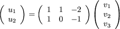
In general, there will be a linear transformation
from the elemental variables to the internal ones. For example in
(2.6), we have